Bounding volumes are an established concept in computer graphics and vision tasks but have seen little change since their early inception. In this work, we study the use of neural networks as bounding volumes. Our key observation is that bounding, which so far has primarily been considered a problem of computational geometry, can be redefined as a problem of learning to classify space into free or occupied. This learning-based approach is particularly advantageous in high-dimensional spaces, such as animated scenes with complex queries, where neural networks are known to excel. However, unlocking neural bounding requires a twist: allowing – but also limiting – false positives, while ensuring that the number of false negatives is strictly zero. We enable such tight and conservative results using a dynamically-weighted asymmetric loss function. Our results show that our neural bounding produces up to an order of magnitude fewer false positives than traditional methods.

We learn neural representations of bounding volumes. The key is a dynamically-weighted asymmetric loss function, which ensures zero false negatives, in order words, no truncated geometry, while keeping false positives minimal for precise bounding. Our approach is adaptable to any dimension and suitable for both point and range queries. It can also be applied to optimise non-neural representations, such as k-DOPs (k discrete oriented polytopes). In results across diverse scenes using 2D, 3D, and 4D queries, our method outperforms traditional bounding methods, achieving up to 10x tighter bounding.

L-R: While AABox, Sphere and kDOP bounding are not tight, Neural - common neural networks - cut off parts of the geometry (see edges of the starfish). Ours Neural - our neural networks - are both tight bounding and conservative (no truncated geometry).

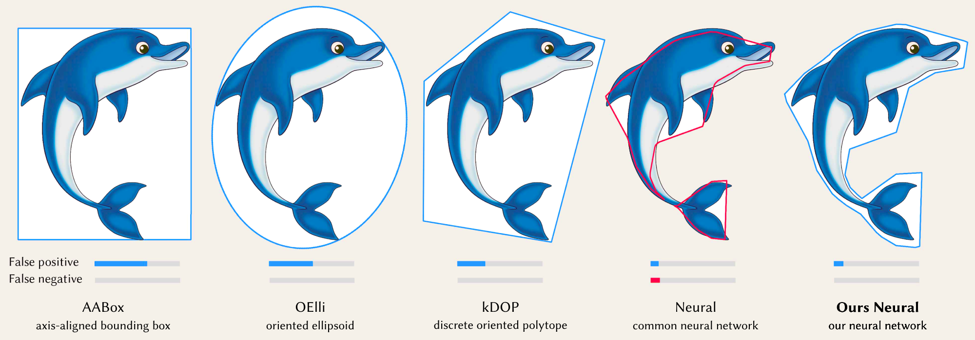
In addition to Ours Neural, our approach can also optimise non-neural representations such as k-DOP, which we call Ours kDOP. The interactive demo below uses 2D point queries to show a comparison of our methods: Ours Neural and Ours kDOP, shown in bold, vs. six baseline methods, on four different objects:

Input is an \(n\)-dimensional indicator function \( f(x) ∈ R^n → \{0,1\} \) that returns 1 inside and on the surface of the object, and 0 everywhere else. To support both point and range queries, on top of the indicator function \( f(x) \), we define a query function \( g(r) ∈ R^n → \{0,1\} \) that is 1 if the indicator function returns 1 for at least one point in the region \( r \). We then approximate \( g(r) \) using another function \( h_{\theta}(r) \) with learnable parameters \( \theta \). The training objective \( L \) is no cost if \( g(r) = h_{\theta}(r) \), otherwise asymmetric costs are applied if false negative: \( g(r) = 1 \) and \( h_{\theta}(r) = 0 \), or false positive: \( g(r) = 0 \) and \( h_{\theta}(r) = 1 \). We approximate \( L \) via a variant of a weighted binary cross entropy loss.

In our implementation, we use small MLPs (Multi-Layer Perceptrons) to achieve faster training and inference. For 2D data, we sample images; for 3D, voxel grids; and for 4D, animated objects are represented as 3D voxel grids stacked in 4D tensors.

We show that our methods generalise across dimensions. Here, we show results for 3D point queries, compared to baseline methods.

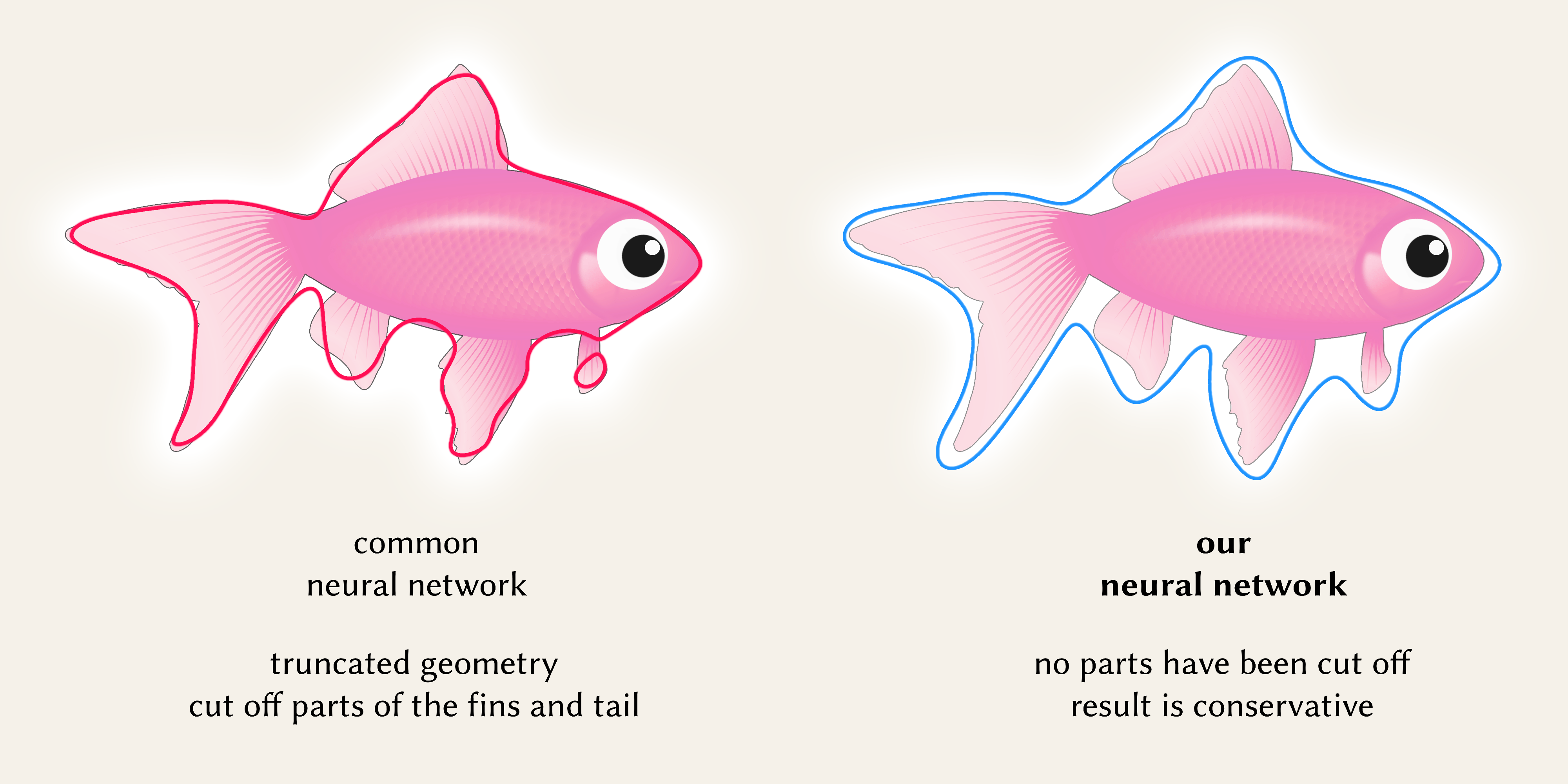
We introduce a variant of our approach that inverts the asymmetric costs associated with false negatives and false positives. Contrasting with our original approach that includes both definite and potential areas, this variant includes only areas that are definitively inside the object, excluding ambiguous regions. This is useful for tasks like sphere tracing where avoiding boundary overestimation is important.

In the following interactive demo, we explore these two types of conservativeness - hit conservativeness, which is the original approach and no-hit conservativeness, which is the variant approach. We show that these two types of conservativeness can be applied in the optimisation of both neural (Ours Neural) and non-neural (Ours kDOP) representations:

@article{liu2023neural,
     title={Neural Bounding},
     author={Liu, Wenxin and Fischer, Michael and Yoo, Paul D. and Ritschel, Tobias},
     year={2023},
     eprint={arXiv:2310.06822},
     archivePrefix={arXiv},
     primaryClass={cs.GR}
}